Introduction: The Evolution of Sequential Learning

Sequential data processing has revolutionized artificial intelligence, enabling machines to understand temporal patterns and dependencies. Three fundamental architectures—RNNs, LSTMs, and GRUs—form the backbone of modern sequence modeling. Each architecture represents a significant evolutionary step in handling sequential information with increasing sophistication.

Understanding Recurrent Neural Networks (RNNs)

RNNs process sequential data by maintaining hidden states that carry information across time steps. The architecture uses a simple feedback mechanism where the current hidden state depends on both the current input and the previous hidden state. This creates a memory effect that allows the network to capture temporal dependencies.

Mathematical Formulation:

h_t = tanh(W_hh * h_{t-1} + W_xh * x_t + b_h)

o_t = W_ho * h_t + b_o

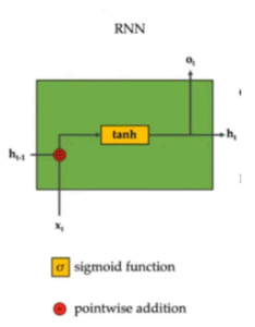
Figure 1: RNN Architecture – The diagram illustrates the basic RNN structure where the hidden state h_{t-1} combines with input x_t through pointwise addition, passes through a tanh activation function, and produces both the current hidden state h_t and output o_t.

The RNN architecture operates on the principle of sharing parameters across time steps, making it parameter-efficient compared to feedforward networks. The tanh activation function squashes the combined input and hidden state into a range between -1 and 1, which helps with gradient flow but can still lead to vanishing gradients in deep temporal sequences. The simplicity of this design makes RNNs computationally efficient, requiring only matrix multiplications and element-wise operations at each time step.

Aspect	Details
Pros	• Simple architecture with minimal parameters • Fast computation and low memory requirements • Easy to implement and understand • Suitable for real-time applications
Limitations	• Vanishing gradient problem for long sequences • Difficulty capturing long-term dependencies • Sequential processing limits parallelization • Gradient explosion issues during training
Applications & When to Use	• Short sequence classification tasks • Simple time series prediction • Real-time streaming data processing • Resource-constrained environments
Use Cases	• Basic sentiment analysis on short texts • Stock price prediction (short-term) • Simple chatbot responses • IoT sensor data processing

Long Short-Term Memory Networks (LSTM)

LSTMs solve the vanishing gradient problem through sophisticated gating mechanisms that control information flow. The architecture introduces three gates—forget, input, and output—along with a cell state that acts as a memory highway. This design enables selective retention and forgetting of information across long sequences.

Mathematical Formulation:

f_t = σ(W_f * [h_{t-1}, x_t] + b_f)     # Forget gate

i_t = σ(W_i * [h_{t-1}, x_t] + b_i)     # Input gate

C̃_t = tanh(W_C * [h_{t-1}, x_t] + b_C)  # Candidate values

C_t = f_t * C_{t-1} + i_t * C̃_t         # Cell state

o_t = σ(W_o * [h_{t-1}, x_t] + b_o)     # Output gate

h_t = o_t * tanh(C_t)                   # Hidden state

 

 

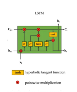
Figure 2: LSTM Architecture – This complex diagram shows the LSTM’s sophisticated gating mechanism with cell state C_t flowing horizontally, three sigmoid gates controlling information flow, and pointwise operations managing selective memory retention.

The LSTM’s architecture represents a significant leap in complexity, with each cell containing approximately four times more parameters than a basic RNN unit. The cell state acts as a conveyor belt, allowing information to flow unchanged across time steps when the forget gate is fully open. The sigmoid activation functions in the gates output values between 0 and 1, effectively acting as filters that determine how much information passes through. This gating mechanism enables LSTMs to learn what to remember, what to forget, and what to output at each time step, making them remarkably effective at capturing long-range dependencies in sequential data.

Aspect	Details
Pros	• Excellent long-term memory capabilities • Solves vanishing gradient problem effectively • Superior performance on complex sequential tasks • Stable training on long sequences
Limitations	• High computational complexity • More parameters require larger datasets • Slower training and inference times • Complex architecture harder to interpret
Applications & When to Use	• Tasks requiring long-term dependencies • Variable-length sequence processing • Complex natural language understanding • Time series with long-range patterns
Use Cases	• Machine translation systems • Document summarization • Speech recognition • Long-term stock market forecasting • Medical diagnosis from sequential data

Gated Recurrent Units (GRU)

GRUs simplify the LSTM architecture by combining forget and input gates into a single update gate while eliminating the separate cell state. This streamlined design maintains LSTM’s effectiveness while reducing computational overhead. The architecture uses reset and update gates to control information flow efficiently.

Mathematical Formulation:

r_t = σ(W_r * [h_{t-1}, x_t] + b_r)     # Reset gate

z_t = σ(W_z * [h_{t-1}, x_t] + b_z)     # Update gate

h̃_t = tanh(W_h * [r_t * h_{t-1}, x_t] + b_h)  # Candidate activation

h_t = (1 – z_t) * h_{t-1} + z_t * h̃_t   # Hidden state

 

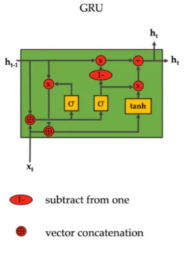
Figure 3: GRU Architecture – The GRU design shows a streamlined approach with reset and update gates working together, featuring the distinctive “1-” operation and simplified gating mechanism that achieves similar performance to LSTMs with fewer parameters.

The GRU architecture cleverly combines the functionality of LSTM’s forget and input gates into a single update gate, reducing the parameter count by approximately 25% while maintaining comparable performance. The reset gate allows the unit to decide how much of the previous hidden state should influence the current candidate activation, effectively controlling the unit’s ability to ignore previous irrelevant information. The update gate determines the balance between retaining old information and incorporating new information, creating a direct interpolation between the previous hidden state and the candidate activation. This design eliminates the need for a separate cell state while preserving the essential gating mechanisms that make LSTMs effective.

Aspect	Details
Pros	• Balanced performance and efficiency • Fewer parameters than LSTM • Faster training and inference • Good performance on medium-length sequences
Limitations	• May underperform LSTM on very long sequences • Less memory capacity than LSTM • Still suffers from sequential processing limitations • Limited control over memory mechanisms
Applications & When to Use	• Medium-length sequence tasks • Resource-constrained applications • Rapid prototyping requirements • When LSTM complexity is excessive
Use Cases	• Sentiment analysis on reviews • Music generation • Short-to-medium text classification • Real-time language translation • Financial time series analysis

Detailed Comparison Analysis

Understanding the nuanced differences between RNN, LSTM, and GRU architectures requires examining multiple dimensions of performance, efficiency, and capability. While each architecture serves specific purposes in sequential learning, their fundamental differences in design philosophy lead to distinct advantages and trade-offs. This comprehensive analysis evaluates these architectures across critical aspects including memory mechanisms, computational requirements, training characteristics, and empirical performance benchmarks to guide practical implementation decisions.

Memory Mechanism Comparison: RNNs use simple hidden states that get overwritten, limiting long-term retention. LSTMs employ sophisticated dual-state systems with explicit memory cells, enabling selective information management. GRUs achieve a middle ground with simplified gating that combines memory functions efficiently.

Computational Complexity Analysis: RNNs require minimal computation (O(n) for sequence length n) but suffer from gradient issues. LSTMs demand the highest computational resources (3x more gates than GRU) with O(4n) complexity. GRUs offer optimal balance with O(3n) complexity, providing 25% fewer parameters than LSTMs.

Training Characteristics: RNN training becomes unstable with increasing sequence length due to gradient problems. LSTM training is stable but requires careful hyperparameter tuning and longer convergence times. GRU training combines stability with efficiency, often converging faster than LSTMs.

Performance Benchmarks: Short sequences: RNN ≈ GRU > LSTM (efficiency matters) Medium sequences: GRU ≈ LSTM > RNN (balance of performance-efficiency) Long sequences: LSTM > GRU > RNN (memory capacity critical)

Conclusion: Making the Right Choice

The evolution from RNNs to LSTMs to GRUs represents progressive refinement in sequential learning architecture design. RNNs provide foundational simplicity but limited capability, LSTMs offer maximum sophistication at computational cost, while GRUs deliver optimal performance-efficiency balance. Modern practitioners should consider task complexity, sequence length, computational constraints, and performance requirements when selecting architectures, with GRUs often serving as the optimal starting point for most applications.